Support Vector Regression (SVR)
- This module explains Support Vector Regression (SVR), including the hyperplane concept, margin, kernel trick, and epsilon-insensitive loss used in regression models.
Hyperplane Concept
What is a Hyperplane?
A hyperplane is a decision boundary used to separate or fit data.
In 2D → it is a line
In 3D → it is a plane
In higher dimensions → it is called a hyperplane
In SVR, the hyperplane is used to fit data such that:
Most data points lie within a certain boundary (margin)
The model remains as flat (simple) as possible
Linear SVR Equation
y=wx+by = wx + by=wx+b
Where:
w = weight (slope)
b = intercept
Margin
Unlike Linear Regression, SVR does not try to minimize total squared error.
Instead, it tries to:
Fit a line where errors within a certain distance are ignored.
This distance is called epsilon (ε).
Margin in SVR
There are two parallel lines:
Upper boundary:
y=wx+b+ϵy = wx + b + \epsilony=wx+b+ϵ
Lower boundary:
y=wx+b−ϵy = wx + b - \epsilony=wx+b−ϵ
The area between them is called the margin (epsilon tube).
Points inside the margin → No penalty
Points outside the margin → PenalizedEpsilon-Insensitive Loss
This is the core concept of SVR.
Idea:
If prediction error is small (within ε), ignore it.
Mathematically:
Loss={0,if ∣y−y^∣≤ϵ∣y−y^∣−ϵ,otherwiseLoss = \begin{cases} 0, & \text{if } |y - \hat{y}| \leq \epsilon \\ |y - \hat{y}| - \epsilon, & \text{otherwise} \end{cases}Loss={0,∣y−y^∣−ϵ,if ∣y−y^∣≤ϵotherwise
Why?
Makes model robust
Focuses only on large errors
Reduces sensitivity to noise
Kernel Trick
Sometimes data is not linearly separable.
In that case, SVR uses Kernel Trick to transform data into higher dimensions.
Instead of explicitly computing new features, kernel functions are used.
Common Kernels
Example
If data looks curved in 2D,
Kernel transforms it into higher dimension
Where it becomes linearly separable.Example (Linear SVR)
Support Vector Regression (SVR) Using Python
This code demonstrates how to use Support Vector Regression (SVR) in Python to model and predict a relationship between variables. The SVR model is trained on sample data, predictions are generated for new values, and the results are visualized using a scatter plot and regression line.
# Step 1: Import Libraries
import numpy as np
import matplotlib.pyplot as plt
from sklearn.svm import SVR

# Step 2: Create Dataset
X = np.array([1, 2, 3, 4, 5]).reshape(-1, 1)
y = np.array([2, 4, 5, 4, 5])

# Step 3: Create SVR Model
model = SVR(kernel='linear', epsilon=0.5)

# Step 4: Train Model
model.fit(X, y)

# Step 5: Predict
X_test = np.linspace(1, 5, 100).reshape(-1, 1)
y_pred = model.predict(X_test)

# Step 6: Plot
plt.scatter(X, y)
plt.plot(X_test, y_pred)
plt.title("Support Vector Regression")
plt.xlabel("X")
plt.ylabel("Y")
plt.show()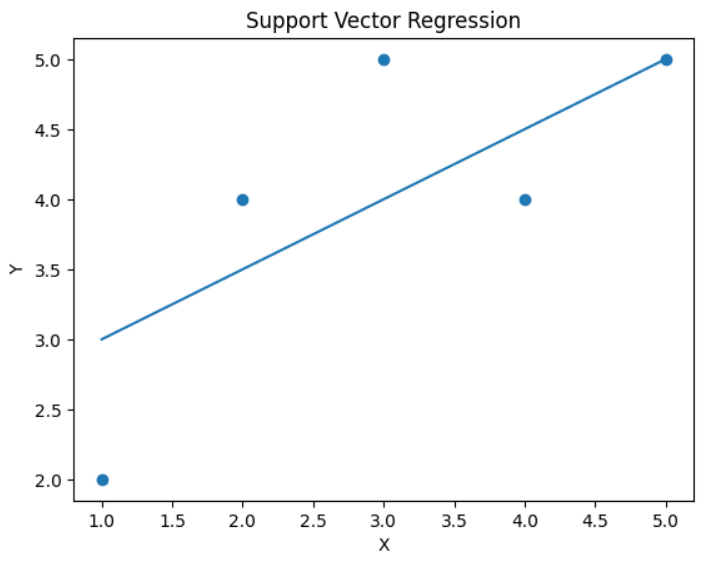
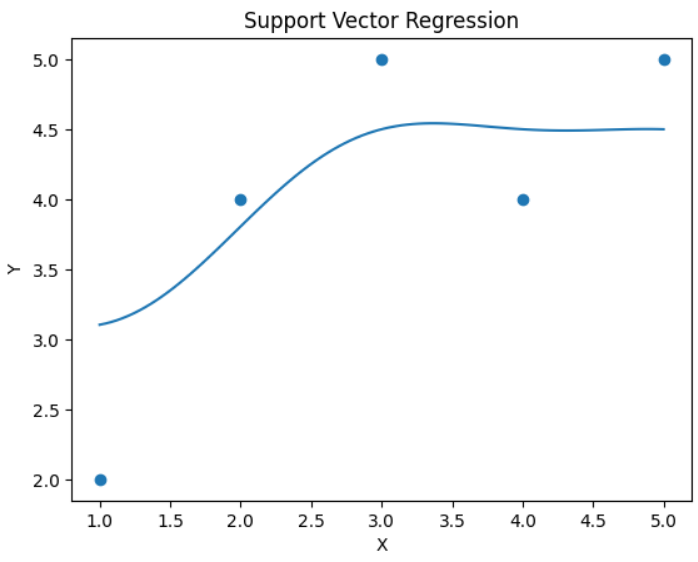
Example with RBF Kernel (Non-Linear)
Support Vector Regression with RBF Kernel
This code creates and trains a Support Vector Regression (SVR) model using the RBF (Radial Basis Function) kernel. The model learns non-linear relationships in the data and fits the training dataset to make predictions.
model = SVR(kernel='rbf', epsilon=0.5)
model.fit(X, y)