Linear Regression
- This module explains Linear Regression in Machine Learning. You will learn simple and multiple linear regression, model assumptions, the cost function (MSE), and how gradient descent is used to optimize the model.
Simple Linear Regression (SLR)
Simple Linear Regression is used when we predict one dependent variable (Y) using one independent variable (X).
Equation
Y=mX+cY = mX + cY=mX+c
m = slope (how much Y changes when X increases by 1 unit)
c = intercept (value of Y when X = 0)
Example
Predicting house price based on area.
Example:
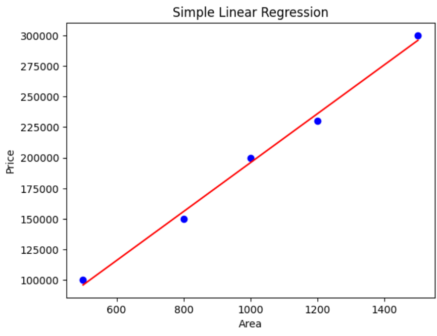
Simple Linear Regression – Area vs Price Prediction
This code demonstrates how to implement Simple Linear Regression using Python. It creates a small dataset of house areas and prices, trains a linear regression model using sklearn, predicts prices, prints the slope and intercept of the regression equation, and visualizes the result with a scatter plot and regression line using matplotlib.
# Step 1: Import Libraries
import numpy as np
import matplotlib.pyplot as plt
from sklearn.linear_model import LinearRegression

# Step 2: Create Dataset (Area vs Price)
# Area (independent variable - X)
X = np.array([500, 800, 1000, 1200, 1500]).reshape(-1, 1)

# Price (dependent variable - Y)
y = np.array([100000, 150000, 200000, 230000, 300000])

# Step 3: Create Model
model = LinearRegression()

# Step 4: Train Model
model.fit(X, y)

# Step 5: Predict
predicted_price = model.predict(X)

# Step 6: Print Equation Values
print("Slope (m):", model.coef_[0])
print("Intercept (c):", model.intercept_)

# Step 7: Plot Graph
plt.scatter(X, y, color='blue')  # actual data
plt.plot(X, predicted_price, color='red')  # regression line
plt.xlabel("Area")
plt.ylabel("Price")
plt.title("Simple Linear Regression")
plt.show()
Output:
Slope (m): 199.99999999999991
Intercept (c): -3999.9999999999127
Multiple Linear Regression (MLR)
Multiple Linear Regression is used when we predict one dependent variable (Y) using multiple independent variables (X1, X2, X3...).
Equation
Y=b0+b1X1+b2X2+b3X3Y = b_0 + b_1X_1 + b_2X_2 + b_3X_3Y=b0+b1X1+b2X2+b3X3
b0b_0b0 = intercept
b1,b2,b3b_1, b_2, b_3b1,b2,b3 = coefficients
Example
Predicting house price based on:
Area
Bedrooms
Age of house
Example:
Multiple Linear Regression – House Price Prediction
This code demonstrates Multiple Linear Regression using Python. It trains a model with multiple independent variables (Area, Bedrooms, and Age) to predict house prices. After training the model using sklearn, it predicts the price of a new house and prints the coefficients (feature impact) and intercept of the regression equation.
import numpy as np
from sklearn.linear_model import LinearRegression

# Independent variables: [Area, Bedrooms, Age]
X = np.array([
    [1000, 2, 5],
    [1500, 3, 3],
    [2000, 4, 2],
    [2500, 4, 1]
])

# Dependent variable: Price
y = np.array([200000, 300000, 400000, 500000])

# Create model
model = LinearRegression()

# Train model
model.fit(X, y)

# Predict price for new house
new_house = [[1800, 3, 2]]
predicted_price = model.predict(new_house)

print("Predicted Price:", predicted_price[0])
print("Coefficients:", model.coef_)
print("Intercept:", model.intercept_)
Predicted Price: 359999.99999999994
Coefficients: [2.00000000e+02 1.45519783e-11 5.92354806e-11]
Intercept: -4.0745362639427185e-10
Assumptions of Linear Regression
Linear Regression works best when these assumptions are satisfied:
1. Linearity
The relationship between X and Y must be linear.
2. Independence
Observations should be independent of each other.
3. Homoscedasticity
Error variance should remain constant across all levels of X.
4. Normality
Errors should be normally distributed.
5. No Multicollinearity (for MLR)
Independent variables should not be highly correlated with each other.
Cost Function (MSE – Mean Squared Error)
The goal of the model is to minimize the error.
Formula
MSE=1n∑(yi−y^i)2MSE = \frac{1}{n} \sum (y_i - \hat{y}_i)^2MSE=n1∑(yi−y^i)2
- yiy_iyi = actual value
- y^i\hat{y}_iy^i = predicted value
Example
If:
Actual value = 80
Predicted value = 75Error = 80 − 75 = 5
Squared error = 25If we have multiple values:
Example:
Mean Squared Error (MSE) – Model Error Calculation
This code calculates Mean Squared Error (MSE) to measure how much the predicted values differ from the actual values.
import numpy as np

actual = np.array([80, 70, 60])
predicted = np.array([75, 72, 58])

mse = np.mean((actual - predicted) ** 2)
print("MSE:", mse)
Output:
MSE: 11.0
Why Squared?
Removes negative values
Penalizes large errors more
Gradient Descent
Gradient Descent is an optimization algorithm used to minimize the cost function.
Working Steps
- Start with random slope and intercept
- Calculate error
- Update slope and intercept
- Repeat until error becomes minimum
Update Formula
m=m−α∂∂mm = m - \alpha \frac{\partial}{\partial m}m=m−α∂m∂
α (alpha) = learning rate
Learning Rate
- Too high → may overshoot minimum
- Too low → training becomes slow
Simple Gradient Descent Example (From Scratch)
Simple Linear Regression – Model Output Explanation
The output shows the values of the regression equation: Slope (m): 1.9896 This means for every 1 unit increase in area, the price increases by approximately 1.99 units. Intercept (c): 0.0304 This is the starting value of price when the area is 0.
import numpy as np
# Data
X = np.array([1, 2, 3, 4])
y = np.array([2, 4, 6, 8])

# Initialize parameters
m = 0
c = 0
learning_rate = 0.01
n = len(X)

# Gradient Descent
for i in range(1000):
    y_pred = m * X + c

    dm = (-2/n) * sum(X * (y - y_pred))
    dc = (-2/n) * sum(y - y_pred)

    m = m - learning_rate * dm
    c = c - learning_rate * dc

print("Slope (m):", m)
print("Intercept (c):", c)
Output:
Slope (m): 1.9896587550255742
Intercept (c): 0.030404521305361965